Table of Contents
Functions are essentially mathematical formulas. They are used to store expressions with variable values, arguments. To execute a function, the values for a number of arguments need to specified. These arguments are then inserted into the expression, making it possible to calculate.
Functions is normally entered in an expression by writing the name followed by arguments, separated by commas (or semicolons in languages with comma as decimal point), in parenthesis, thus following the syntax name(arg1, arg2, ...). Qalculate! will give a helpful error message if the arguments are not correct.
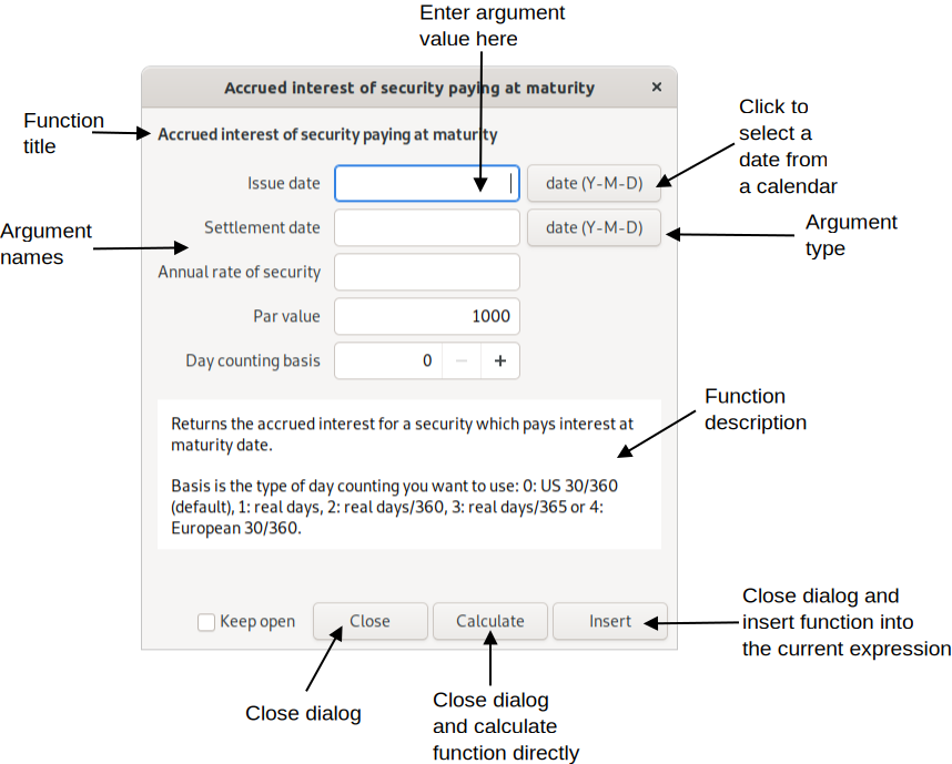
The insert function dialog presents an easy way to insert a function and its arguments.
Although it can lower the readability of an expression, it is perfectly legal to skip the parenthesis and put the arguments after a space, and end with a space or operator. This is most useful in short expressions with single argument functions (e.g. “sqrt 5”).
Argument types include:
-
Free — anything
-
Number — a numeric value
-
Integer — a whole number
-
Symbol — a defined or undefined unknown variable
-
Text — a free text string
-
Date — a date in local or standard format (Year-Month-Day, recommended)
-
Vector
-
Matrix
-
Boolean — 0 for false, 1 for true
-
Object — the name of a variable, function or unit
-
Variable — the name of a variable
-
Function — the name of a function
-
Unit — the name of a unit
-
File — the path to a file
-
Angle — an angle used in trigonometric functions, meaning a number and an angle unit. If no angle unit is included the default is used.
The argument can be restricted by further conditions. For example that a number must be positive.
Most arguments (primarily number arguments) can be replaced by a vector. The function will then be calculated for each vector element and a new vector will be returned. If more than one argument are supplied to a function that takes exactly one argument, each argument will be treated as elements of a vector.
Here the main function categories and some of their members are described, to give an overview of available functions. For information about separate functions and a complete list of all available functions see Appendix A, Function List or the function manager.
- Algebra
-
Contains sum() and product(), which corresponds to the sum and product signs. solve() solves equations (e.g. “solve(x × 2 = 8)” returns “4” meaning that x equals 4). Use solve2() and multisolve() to solve multiple equations with multiple variables.
- Calculus
-
Includes diff(), which calculates the derivative of an expression with optional arguments “with respect to” (default x) and “order” (default 1), and a limited integration function.
- Combinatorics
-
Contains functions such as perm() for permutations, comb() for combinations, and factorial().
- Comblex Numbers
-
Contains functions useful for calculations with complex numbers, including arg() for principal argument and conj() for conjugate.
- Data Sets
-
A data set consists of a set of properties and objects, which can be accessed by a function which takes two arguments — object and property. The function returns the object's value for the selected property. For example, the data in the “Elements” data set is accessed with the atom() function, with the element (referenced using atomic symbol, number or name) and property (e.g. weight) as arguments. The special property “info” displays all properties of the object in a dialog window.
- Date & Time
-
Includes days() and yearfrac() which returns the number of days and fractional years, respectively, between two dates.
- Exponents & Logarithms
-
Standard logarithmic and exponential functions. ln() calculates the natural logarithm of a number, while log() allows a choice of base as the second argument. The cbrt() and root() functions only calculates real roots. For roots of odd degree the root functions give a different answer than the exponential operator, “^”, for negative values (“cbrt(-8) = -(8)^(1/3) = -2”, but “(-8)^(1/3) = 1 + 1.73i”).
- Economics
-
This essentially includes most of the financial functions that are usually found in spreadsheet applications.
- Elements
-
This category includes functions to retrieve data such as atomic weight. The atom() function opens a window with available data of an element. These functions accept the number, symbol or name of the element as argument. The data are loaded on demand.
- Geometry
-
Category with formulas mostly for calculation of circumference, area and volume of geometric shapes.
- Logical
-
Some procedural functions mainly for use in other functions. These include if(), which tests a conditional expression and returns a value depending on if the expression evaluates true or false, and for(), which processes a value while a condition is true.
- Matrices & Vectors
-
These are functions that generate, access and process matrices and vectors. The vector() function generates a vector from a variable number of arguments for elements, while matrix() first needs the number of rows and columns and then the elements from left to right. Matrices can also be imported directly from a CSV file with load().
Separate elements at a specified row and column are accessed with element(). Other functions include det() for calculation of the determinant of a matrix and inverse() which returns the inverse of the given matrix, as well as functions such as sort() and rank().
- Miscellaneous
-
A category for functions that do not fit elsewhere.
- Number Theory
-
Contains subcategories arithmetic, number bases, and rounding, in addition to functions such as abs(), which returns the absolute value of a number (“|” can also be used; e.g. “|-5| = abs(-5) = 5”, and gcd(), the greatest common divisor. round() is the standard rounding function (note that halfway numbers are rounded to even). The functions for number bases translates a text string, representing an expression with numbers in a different base, to a decimal number. Includes bin() for binary numbers, hex() for hexadecimal numbers, oct() for octal numbers and base() for numbers in a any other base.
- Special Functions
-
Includes beta(), gamma() and similar functions, as well as Riemann zeta (zeta()) and Kronecker delta (kronecker()).
- Statistics
-
Contains a lot of functions for descriptive statistics and some statistical tests. Data sets are stored as vectors. Generally, functions with a vector/data set as last argument can take elements/samples as a variable number of arguments directly instead of in a vector (e.g. “mean(1, 2, 3)” equals “mean(vector(1, 2, 3))”). Also contains the rand() function, which returns a pseudo random number between 0 and 1 (with no argument, or zero), or a random integer between one and the specified number.
- Trigonometry
-
Trigonometric functions, including sin(), cos(), tan(), sec(), csc(), cot(), and hyperbolic and inverse versions of those. These functions take as argument an angle. If the default angle unit ( → ) is set to none, the argument must have an angle unit appended (degrees, radians or gradians), otherwise the default unit will be appended automatically (and removed from result of inverse functions).
- Utilities
-
Various utility functions. Most are only useful in definition of other functions. The save() function can however be a quick way of storing a value in a variable, and csum() can be a powerful tool for data processing. This category also contains some functions, such as char() and ascii(), that might be useful for programmers. , replace() provides an easy way of replacing unknown variables by known expressions in a value (e.g. “replace(5x^2 + x, x, 3)” equals “5 × 3^2 + 3”).
Functions are a bit more complex than variables, but can nevertheless be relatively easily created. Select → → or → → ), or click the on the keypad or in the function manager and a function edit dialog pops up. There are two different dialogs for function creation.
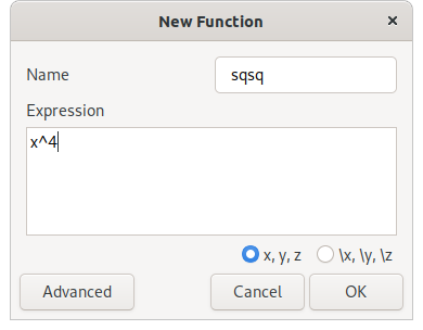
The simple function edit dialog only allows entry of a single name and an expression. You have here the option to use x, y and z with or wihout (default) a backslash for argument placeholders in the expressions. The expression “x^4” then creates a function which calculates the fourth power of a single argument. If you name it for example “sqsq”, “sqsq(2)” will calculate “2^4”. The use of \x, \y, \z avoid any possible conflict with variables, units and functions. When you edit an existing function, it will use the notation with backslash.
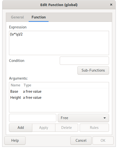
The advanced dialog, with access to all function properties, consists of two tabs/pages; the first with general descriptive information and the last for the function definition. First enter a name, used to reference the function in an expression. If an expression is entered a bit further down, then the function will already be fully working. A bit more does however need to be said about the function expression.
The expression of a function is basically a normal expression with placeholders for arguments. These placeholders consists of a backslash and a letter — x, y, z for the 1st, 2nd and 3rd arguments and a to u for argument 4 to 24. They are replaced by entered arguments when a function is calculated. The placeholders naturally also decide the number of arguments that a function requires. For example the function for triangle area (“base × height / 2”) has the name triangle and the expression “(\x × \y)/2”, which gives that “triangle(2, 3)” equals “(2 × 3) / 2” and returns “3” as result. An argument can be used more than one time and all arguments must not necessarily be in order in the expression.
Additionally, optional arguments can be put in the expression with upper-case (X, Y, Z, ...) instead of lower-case letters (x, y, z, ...). The default value can be put in brackets after the letter (e.g. “\X{2}”). The default value may be omitted and is then zero. All additional arguments after an optional argument must also be optional.
A condition that must be true (>0) for the function to be calculated, can optionally be entered in the text field below the expression. This follows the same conventions as function expressions. For example if the second argument must be higher than the first, “\y > \x” may be entered as condition.
Further, name, type and condition for each argument can be specified.
To keep functions well organized, supply a category, descriptive name and description. A function can also hidden from menus with the corresponding check box, which can be useful for sub functions.
Global, system-wide functions can not actually be changed by the user, but if one of these functions is edited, they are deactivated and seemingly replaced by a new function. This way global functions can be “deleted” by deactivation. Some functions are however hard-coded and cannot be changed by the user.


